Is there such a thing as a sexy ZIP code demographic to a Liquor Store?
This week’s assignment was a group effort with 2 other classmates, Jocelyn and Joshua.
The project was designed to build upon our existing proficiency with Data Wrangling using Python pandas library and fortify our statistical fundamentals including Linear Regressions and Cross Validation using different Linear Models.
Specifically the project required us to:
- explore a large public governmental dataset of Liquor Sales in Iowa for 2015
- work towards the goal of recommending potential locations for Liquor Stores in the state
- clean the data, as necessary
- consider the introduction of supporting datasets such as Demographics
- develop a reproducible method supported by sound practices for making location recommendations
- utilize visual and statistical to present our recommendations
- use new statistical tools and functions such as RidgeCV, LassoCV for modeling predictive values based on provided features
Project 3 Jupyter Notebook - Group Submission
Note: The methodology below is drawn from the “Data Science Workflow” document provided by General Assembly
IDENTIFY THE PROBLEM
We’ve been tasked with making recommendations on where to open new liquor stores in the state of Iowa based on a dataset of the Iowa State Liquor Authority acting as a “Wholesaler” from 2015
Risks and Assumptions
It was determined early on that the data presented did not represent consumer retail sales, but rather sales from the State to the Liquor Stores. Therefore, we could not directly infer any profitability at the store level directly.
We made the assumption that the sales data was reasonably accurate as we had no way to independently audit the entries. We also assumed that the ZIP code for the stores was accurate, although we were able to catch several dozen obvious systemic errors, but the percentage was very small given that there 2.7-million records.
Because we had no information regarding the end user sale to the consumer, we made the assumption that every bottle purchased from the State was sold within a very short period of time.
We added to the Liquor dataset, a dataset of 2010 demographic data obtained from the Iowa data website here. We likewise assume that this data is generally accurate and that there are no gross errors on it’s face. Of course, demographic data can be biased at the collection level.
ACQUIRE THE DATA
The 2015-2016 Iowa Liquor Sales database is available on the data.iowa.gov website here . It consists of 2,709,552 records of transactions of sales which took place between the state of Iowa and individual liquor stores. In Iowa, the state itself acts as the wholesaler.
The census-2000 demographic data which we incorporated was extensive and consisted of several different demographic segments including age, housing, income, race, and poverty level. All of which can be considered when determining a location for Liquor stores.
A full description of the liquor dataset can be found below.
- Name: Iowa_Liquor_Sales_reduced.csv
- Delimiter: “,”
- Records: 2,709,552
- Sources: Iowa Department of Commerce, Alcoholic Beverages Division
-
Columns:
- Date - unique row ID - integer
- Store Number - unique ID for liquor store - integer
- City - city in which store located - string
- Zip Code - zip code in which store located - string
- County Number - IOWA county number in which store located - integer
- County - IOWA county name in which store located - string
- Category - numerical category for liquor type - integer
- Category Name - text name for liquor type - string
- Vendor Number - unique id for supplier to state - integer
- Item Number - unique id for actual product sku - integer
- Bottle Volume (ml) - size in ml of bottle - integer
- State Bottle Cost - cost from the supplier to the state - float
- State Bottle Retail - cost from the state to the store - float
- Bottles Sold - quantity of bottle sold - integer
- Sale (Dollars) - total sale of this transaction - float
- Volume Sold (Liters) - total volume of this transaction in liters - float
- Volume Sold (Gallons) - total volume of this transaction in gallons - float
PARSE THE DATA
Although data was available to us for years from 2012-2016, we focused only on the 2015 data as a reasonable measure of yearly sales and because it was a manageable size. The full dataset from 2012-2016 was over 2.7GB and we didn’t have the resources to deal with such a large load as that. The 2015 sample was 360MB and was far easier to work with for the purposes of this project.
We read the liquor sales data in with python pandas library from a csv file. The csv file we were presented was cleaned somewhat from the source files at data.iowa.gov. Specifically, they had the “Store Location” field dropped. The “Store Location” field contained \n linebreaks which may have led to undesirable parsing results.
We compiled from a few other sources a master lookup reference of ZIP, COUNTY, COUNTY#, CITY, ZIP-AREA-SQKM which we used to join against our liquor database and fill in any erroneous or missing data for those liquor fields.
This master zip-code-database file also contained the geographic area for the particular zip code in units of square meters. We did not that there are now more zip codes in the state than we had unique geographic area for. It seems that some larger zip codes were split into 1 or more smaller zip codes sometime since the area data was compiled. This should not affect our model since we are using the geographic area simply as a point of information in our results and not as an input to our model.
MINE THE DATA
Our overall goal is to develop a model to recommend zip codes which are best performing based on 2 target metrics.
1) Maximum Total Overall Sales in Dollars for the Zip code and
2) Maximum Total Volume Sold in Liters for the Zip Code
In order to obtain model to predict the 2 targets above, we utilized, exclusively the demographic features which we had joined to our liquor dataset by zip code.
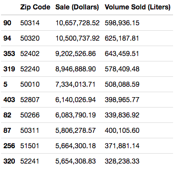
Before performing any aggregation or discarding any outliers, we took a snapshot to see which zip codes had the highest yearly total sales.
Prior to performing significant modeling efforts, we needed to first perform a bit of cleanup and aggregation on the initial data.
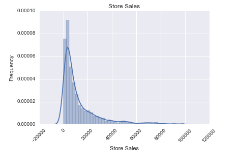
We noticed that there were a very small number of very large “distributer” stores. We recognized them as significant outliers and trimmed them by setting our threshold for exclusion to be any stores with greater than $100,000 in yearly sales. This threshold was arrived at by visual inspection of the following histogram.

Once we had trimmed outlier stores we still had a skewed distribution, however, we were comfortable with the 1 order of magnitude shorter tail. (see below)
After the elimination of the outlier stores, we went on to aggregate total sales and total volume on the zip code level for all stores. As noted above, these would be our targets for our model.
# Aggregate sales and volume by zip code
store_aggs = ['Store Sales', 'Store Volume']
zip_summary = df3.groupby('Zip Code')[store_aggs].sum().reset_index().dropna()
zip_summary.columns = ['Zip Code', 'Zip Sales - Total', 'Zip Volume - Total']
zip_aggs = ['Zip Sales - Total', 'Zip Volume - Total']
We have now arrived at these Top performing Actual Zip Codes based on Total Yearly Sales:

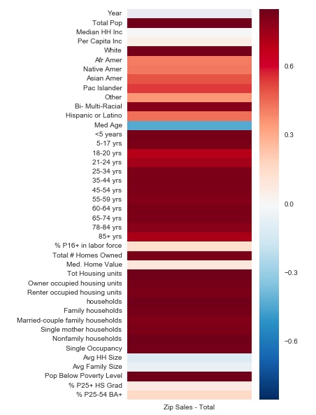
In an effort to understand how our demographic data may be correlated with our targets, we created a heat map for each. You should notice that they depict an nearly identical correlation map for both targets. This should be intuitive because Sales should be directly proportional to Volume sold.
| Sales | Volume |
|---|---|
 |
 |
When looking at the heatmaps while sorted by the correlation figure, a few unexpected features rise to the top. Namely, population of persons “<5 years old” and “# of owner-occupied housing units”. While median household income seems to be very weakly correlated.
| Sales (Sorted) | Volume (Sorted) |
|---|---|
 |
 |
REFINE THE DATA
We have already mentioned above that we chose to eliminate outlying stores based on a sales threshold of $100K. We then aggregated our targets of total sales and total volume.
In addition to these manipulations, we also aggregated total number of stores per zip code.
Two other fields were computed at this point which will be used during our recommendation phase.
- Sales Dollars per Liter - was derived to denote whether a zip code should be considered an expensive, average or inexpensive liquor market.
- Stores per Sq Kilometer - was derived to give a sense of whether the market was oversaturated with Liquor stores or whether there was a potential for more supply.
BUILD A DATA MODEL
With our targets ready and our demographic features data in hand, we set out to build 2 separate models. For each we used LassoCV (with our cv argument set at 5) in order to assist in elimination of features that the algorithm deemed as unimportant.
X = model_df[features]
y_sales = model_df['Zip Sales - Total']
lasso = linear_model.LassoCV(cv=5)
model_sales = lasso.fit(X,y_sales)
print 'r-squared: {}'.format(model_sales.score(X,y_sales))
print 'alpha applied: {}'.format(model_sales.alpha_)
X = model_df[features]
y_volume = model_df['Zip Volume - Total']
lasso = linear_model.LassoCV(cv=5)
model_volume = lasso.fit(X,y_volume)
print 'r-squared: {}'.format(model_volume.score(X,y_volume))
print 'alpha applied: {}'.format(model_volume.alpha_)
| Sales | Volume |
|---|---|
 |
 |
| - an r-squared value of: 0.816989065682 | - an r-squared value of: r-squared: 0.803698824346 |
| - an alpha applied value of: 3512.74084712 | - an alpha applied value of: 237.245609349 |
It’s interesting to note that some of the features that the heatmap picked up as highly correlated received a very large coefficient in our models: - age < 5 : 2nd highest ranked coefficient: 1,781,072.90 - Owner occupied housing units: 4th highest ranked coefficient 959,592.22
Whereas “Total # Homes Owned” received a coefficient value of 0.00, suggesting that it is not important in determining either of our targets.
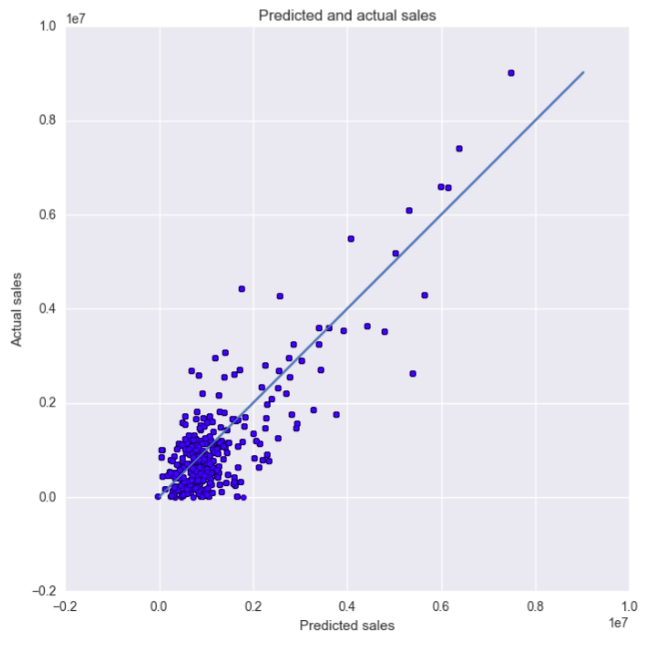
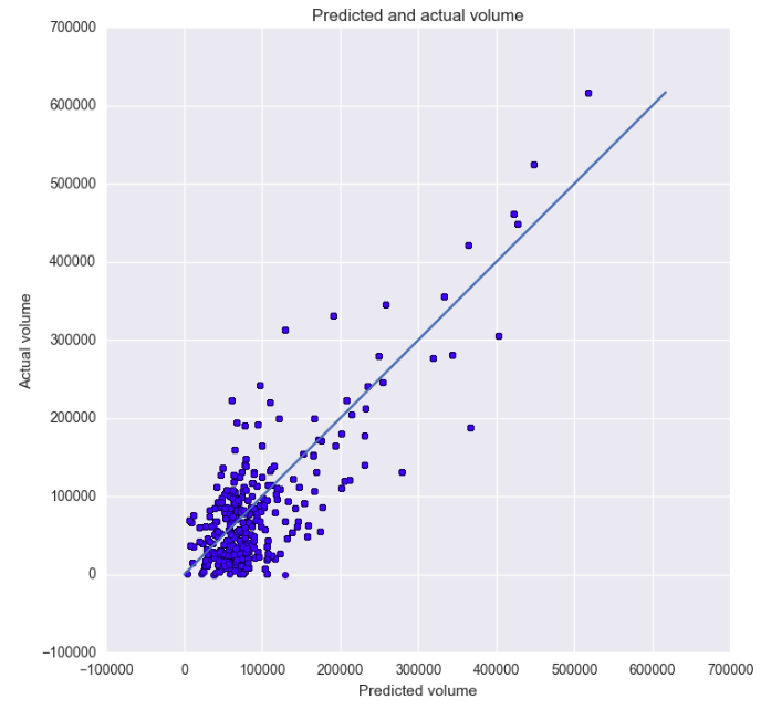
As you can see from the plots above, our model does a fairly decent job of predicting the yearly sales given a set of demographic data for a zip code. We were please with this result and continued our efforts.
Rather than utilize a train-test-split or other method to extrapolate our predictions, we felt that the best idea would be to consider the zipcodes that had at least 1 store in them (n=362) vs. the zipcodes that had 0 stores in them (n=459). In doing so, we are now running our model against zipcodes that can be characterized by the demographic data but do not yet contain a liquor store.
Once we ran our models and found their predictions we again sorted our results by Total Yearly Sales with the expectation that based on the demographics of the zip code, these were the strongest contenders for opening future stores.
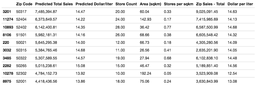
Several of our predicted zip codes duplicated zip codes which we found earlier in this write up, however a few new zip codes have emerged: 52001, 52302, 50265, 50322, 50315, 50021, 52402
According to the mode’s predictions, based on the zip code’s demographic characteristics, these are all highly attractive markets for expansion. However, please be aware that 52403 already has a a relatively high saturation of stores/sqkm. Additionally, 52001 and 52302 both have relatively low dollars / litre and this suggest that the zip may be less likely to support a higher end, more expensive store.
On the map below are the top 10 zip codes which represent the places which our model predicts the highest Total Yearly Sales. It is showing the details for the highest rated zip code, 50317

FURTHER WORK
The budget for our data acquisition did not allow us to obtain demographic data newer than the 2000 census, we would highly recommend that more current data be sought to perhaps more accurately reflect current demographic characteristics.
There were a few other questions which arose from the project. We struggled with the fact that our model predicted negative total sales and volume and we’d like to further investigate why that is.
In addition, we’d like to better understand the actual price to the consumer at each store to better understand where the most PROFITABLE stores are located, not simply the stores that are spending the most on purchasing inventory (which is essentially what we’ve done).
We’d like to better understand if our assumptions made about inventory to sale is reasonable. Perhaps look at whether we can determine areas for socially responsible outreach regarding drinking responsibly.
Can we geocode the stores to a more granular scale and consider the actual commercial areas they reside in? Can we interpolate an optimum mix of products? Can we make decisions about ramping up stock based on seasons?
POSTSCRIPT
There are many ways to approach the problem of recommending locations for expansion. Certainly there are professional consultant teams with the sole responsibility of doing this type of analysis for corporate expansion. We chose an approach that made sense to us given the data available. We feel confident that there are some valid results which can be drawn from our decisions. But we are also aware that there may be certain aspects and variables which we didn’t consider or things that we did include that we shouldn’t have.
These are the some of the big questions which face the Data Scientist. To be able to see the various angles, understand the relationships, consider the implications of their decisions. They need to be able to support and defend their approach. They need to create a method which can be tweaked, tuned and reproduced.
These are the struggles. These are a few of the driving forces behind my interest in becoming a productive member of the Data Science community.